How to Find Seasonality Patterns in Time Series

In my skilled life as an information scientist, I’ve encountered time sequence a number of instances. Most of my data comes from my tutorial expertise, particularly my programs in Econometrics (I’ve a level in Economics), the place we studied statistical properties and fashions of time sequence.

Among the many fashions I studied was SARIMA, which acknowledges the seasonality of a time sequence, nonetheless, we’ve by no means studied methods to intercept and acknowledge seasonality patterns.

More often than not I needed to discover seasonal patterns I merely relied on visible inspections of information. This was till I came across this YouTube video on Fourier transforms and finally discovered what a periodogram is.

On this weblog publish, I’ll clarify and apply easy ideas that may flip into helpful instruments that each DS who’s finding out time sequence ought to know.

Desk of Contents

1. What’s a Fourier Remodel?
2. Fourier Remodel in Python
3. Periodogram

Overview

Let’s assume I’ve the next dataset (AEP energy consumption, CC0 license):

import pandas as pd
import matplotlib.pyplot as plt

df = pd.read_csv("knowledge/AEP_hourly.csv", index_col=0) 
df.index = pd.to_datetime(df.index)
df.sort_index(inplace=True)

fig, ax = plt.subplots(figsize=(20,4))
df.plot(ax=ax)
plt.tight_layout()
plt.present()

It is vitally clear, simply from a visible inspection, that seasonal patterns are taking part in a task, nonetheless it could be trivial to intercept all of them.

As defined earlier than, the invention course of I used to carry out was primarily guide, and it might have seemed one thing as follows:

fig, ax = plt.subplots(3, 1, figsize=(20,9))

df_3y = df[(df.index >= '2006–01–01') & (df.index = '2006–01–01') & (df.index = '2006–01–01') & (df.index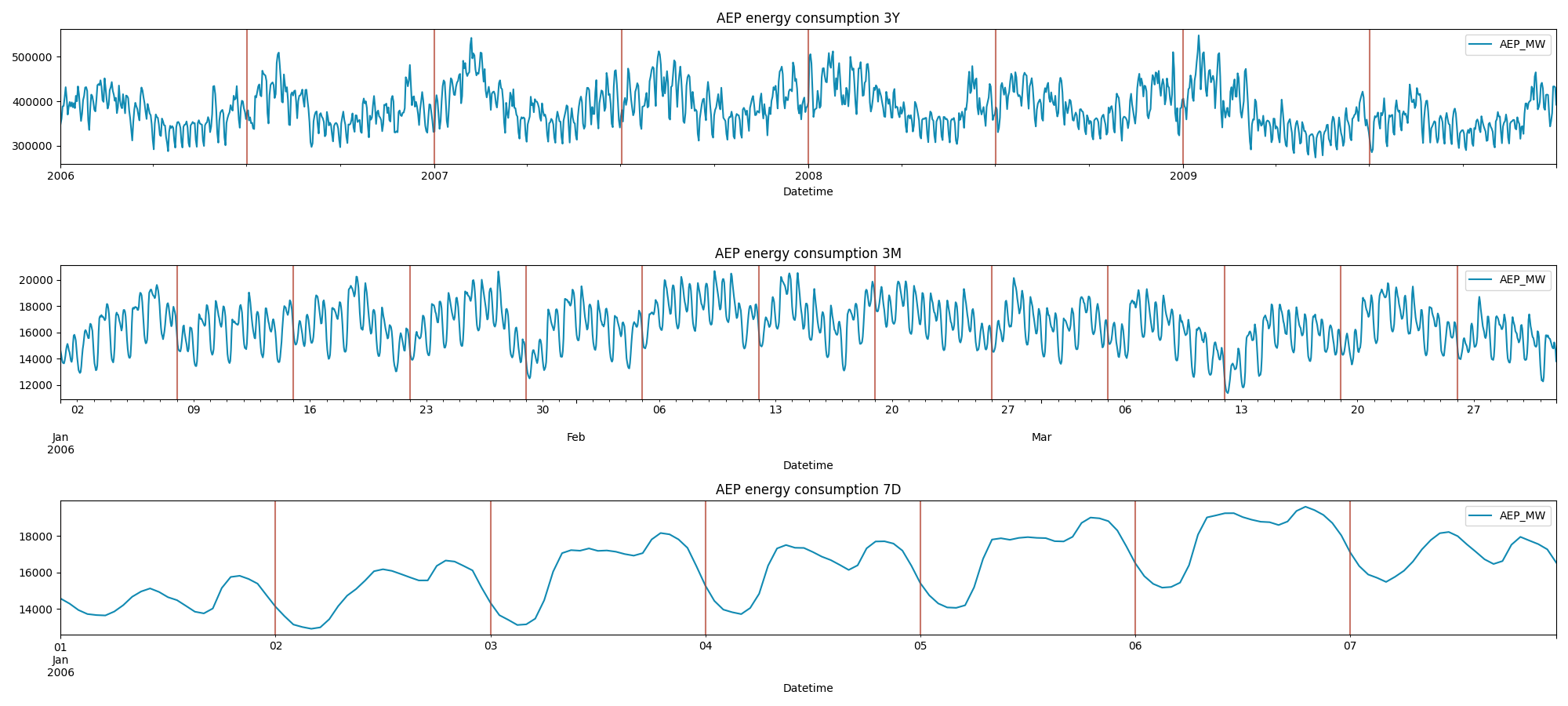 

This is a more in-depth visualization of this time series. As we can see the following patterns are influencing the data: **- a 6 month cycle,

• a weekly cycle,
• and a daily cycle.**

This dataset shows energy consumption, so these seasonal patterns are easily inferable just from domain knowledge. However, by relying only on a manual inspection we could miss important informations. These could be some of the main drawbacks:

• Subjectivity: We might miss less obvious patterns.
• Time-consuming : We need to test different timeframes one by one.
• Scalability issues: Works well for a few datasets, but inefficient for large-scale analysis.

As a Data Scientist it would be useful to have a tool that gives us immediate feedback on the most important frequencies that compose the time series. This is where the Fourier Transforms come to help.

1. What is a Fourier Transform

The Fourier Transform is a mathematical tool that allows us to “switch domain”.

Usually, we visualize our data in the time domain. However, using a Fourier Transform, we can switch to the frequency domain, which shows the frequencies that are present in the signal and their relative contribution to the original time series.

Intuition

Any well-behaved function f(x) can be written as a sum of sinusoids with different frequencies, amplitudes and phases. In simple terms, every signal (time series) is just a combination of simple waveforms.

Where:

• F(f) represents the function in the frequency domain.
• f(x) is the original function in the time domain.
• exp(−i2πf(x)) is a complex exponential that acts as a “frequency filter”.

Thus, F(f) tells us how much frequency f is present in the original function.

Example

Let’s consider a signal composed of three sine waves with frequencies 2 Hz, 3 Hz, and 5 Hz:

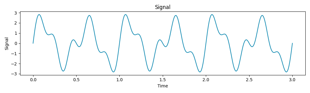
Now, let’s apply a Fourier Transform to extract these frequencies from the signal:

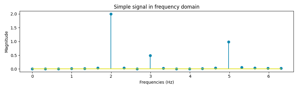
The graph above represents our signal expressed in the frequency domain instead of the classic time domain. From the resulting plot, we can see that our signal is decomposed in 3 elements of frequency 2 Hz, 3 Hz and 5 Hz as expected from the starting signal.

As said before, any well-behaved function can be written as a sum of sinusoids. With the information we have so far it is possible to decompose our signal into three sinusoids:

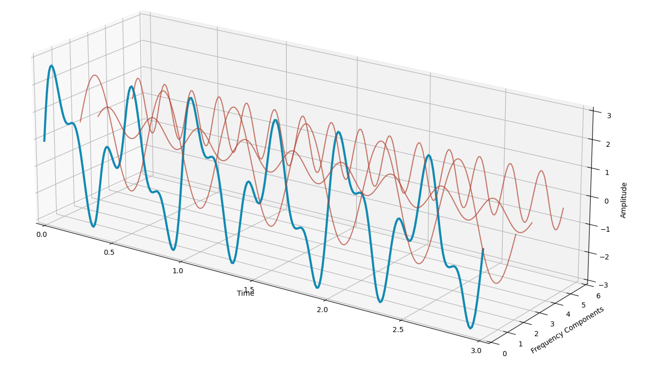
The original signal (in blue) can be obtained by summing the three waves (in red). This process can easily be applied in any time series to evaluate the main frequencies that compose the time series.

2 Fourier Transform in Python

Given that it is quite easy to switch between the time domain and the frequency domain, let’s have a look at the AEP energy consumption time series we started studying at the beginning of the article.

Python provides the “numpy.fft” library to compute the Fourier Transform for discrete signals. FFT stands for Fast Fourier Transform which is an algorithm used to decompose a discrete signal into its frequency components:

from numpy import fft

X = fft.fft(df['AEP_MW'])
N = len(X)
frequencies = fft.fftfreq(N, 1)
durations = 1 / frequencies
fft_magnitude = np.abs(X) / N

masks = frequencies >= 0

# Plot the Fourier Remodel
fig, ax = plt.subplots(figsize=(20, 3))
ax.step(durations[mask], fft_magnitude[mask]) # Solely plot constructive frequencies
ax.set_xscale('log')
ax.xaxis.set_major_formatter('{x:,.0f}')
ax.set_title('AEP vitality consumption - Frequency-Area')
ax.set_xlabel('Frequency (Hz)')
ax.set_ylabel('Magnitude')
plt.present()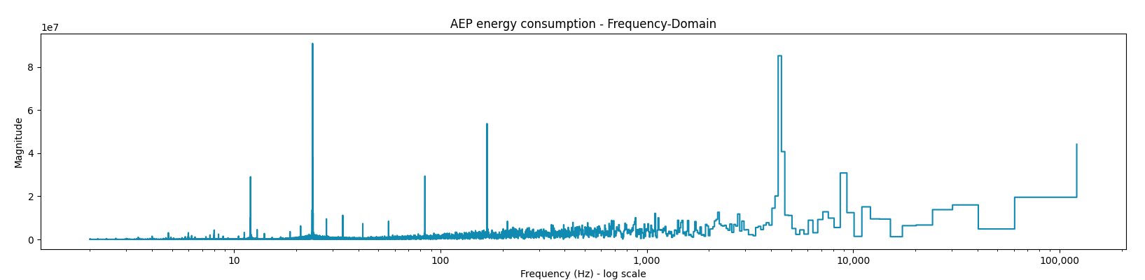

That is the frequency area visualization of the AEP_MW vitality consumption. After we analyze the graph we will already see that at sure frequencies we’ve the next magnitude, implying greater significance of such frequencies.

Nevertheless, earlier than doing so we add yet one more piece of principle that may enable us to construct a periodogram, that may give us a greater view of an important frequencies.

3. Periodogram

The periodogram is a frequency-domain illustration of the energy spectral density (PSD) of a sign. Whereas the Fourier Remodel tells us which frequencies are current in a sign, the periodogram quantifies the facility (or depth) of these frequencies. This passage is usefull because it reduces the noise of much less essential frequencies.

Mathematically, the periodogram is given by:

The place:

• P(f) is the facility spectral density (PSD) at frequency f,
• X(f) is the Fourier Remodel of the sign,
• N is the entire variety of samples.

This may be achieved in Python as follows:

power_spectrum = np.abs(X)**2 / N # Energy at every frequency

fig, ax = plt.subplots(figsize=(20, 3))
ax.step(durations[mask], power_spectrum[mask])
ax.set_title('AEP vitality consumption Periodogram')
ax.set_xscale('log')
ax.xaxis.set_major_formatter('{x:,.0f}')
plt.xlabel('Frequency (Hz)')
plt.ylabel('Energy')
plt.present()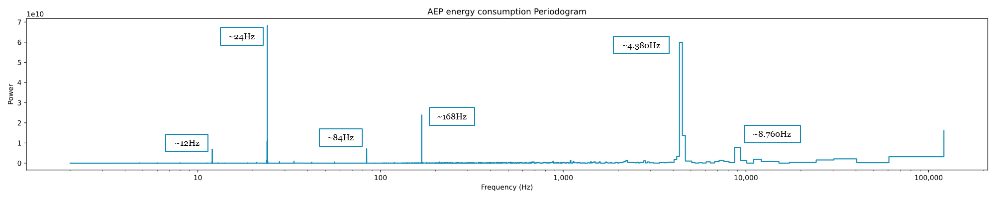

From this periodogram, it’s now doable to draw conclusions. As we will see essentially the most highly effective frequencies sit at:

• 24 Hz, comparable to 24h,
• 4.380 Hz, corresponding to six months,
• and at 168 Hz, comparable to the weekly cycle.

These three are the identical Seasonality parts we discovered within the guide train executed within the visible inspection. Nevertheless, utilizing this visualization, we will see three different cycles, weaker in energy, however current:

• a 12 Hz cycle,
• an 84 Hz cycle, correspondint to half per week,
• an 8.760 Hz cycle, comparable to a full yr.

It’s also doable to make use of the operate “periodogram” current in scipy to acquire the identical end result.

from scipy.sign import periodogram

frequencies, power_spectrum = periodogram(df['AEP_MW'], return_onesided=False)
durations = 1 / frequencies

fig, ax = plt.subplots(figsize=(20, 3))
ax.step(durations, power_spectrum)
ax.set_title('Periodogram')
ax.set_xscale('log')
ax.xaxis.set_major_formatter('{x:,.0f}')
plt.xlabel('Frequency (Hz)')
plt.ylabel('Energy')
plt.present()

Conclusions

After we are coping with time sequence some of the essential parts to contemplate is seasonalities.

On this weblog publish, we’ve seen methods to simply uncover seasonalities inside a time sequence utilizing a periodogram. Offering us with a simple-to-implement instrument that may turn into extraordinarily helpful within the exploratory course of.

Nevertheless, that is simply a place to begin of the doable implementations of Fourier Remodel that we may gain advantage from, as there are a lot of extra:

• Spectrogram
• Characteristic encoding
• Time sequence decomposition
• …

Please depart some claps if you happen to loved the article and be happy to remark, any suggestion and suggestions is appreciated!

_Here you can find a notebook with the code from this blog post._